| Santa Monica Bay Nearshore Zone A. Kimo Morris |
updated: 1/07/06
|
||||||||||||||||||||
|
|
|||||||||||||||||||||
|
|||||||||||||||||||||
 Graduate work of A. Kimo Morris
|
D = log10(h/u3)
|
Equation 3-1
|
where the stratification parameter (D) equals the log of the ratio of the depth (h) to the water velocity (u) cubed. Small values of D indicate vertically well-mixed water. This general equation explains mixing best for wide linear coastlines where surface and tidal waves approaches the beach perpendicular to shore, as is the case near Dockweiler Beach, Santa Monica Bay. 
This phenomenon can potentially generate a very interesting feature nearshore. The area inside and outside the threshold (for the purposes of this proposal will be termed inshore and offshore, respectively) will have different physical characteristics. For example, because of the mixing described above, the water mass will remain a uniform density, temperature and salinity. Also, this zone will have higher turbidity because of sediment stirring and a greater concentration of dissolved oxygen. Interestingly, tidal mixing in the nearshore can also result in intense phytoplankton blooms (Pingree et al., 1975), which were prevalent throughout southern California, including Santa Monica Bay, during the late summer of 2003. In contrast, the offshore water mass can be stratified, with vertical profile gradients and less turbidity. This can create a steep density gradient at the mixing threshold that could be further enhanced by cabbeling, a phenomenon where two adjacent water masses of differing temperature and/or salinity, but which have identical densities, mix forming a denser parcel of water than either of the two original water masses (Beer, 1983). Cabbeling would likely be a means by which the resulting front could persist, where any water resulting from mixing across the boundary would sink, thus helping to maintain the discontinuity.
Further offshore, where bottom depth does not influence mixing, tidal flow can also result in complete mixing of the water column if there is sufficient difference between high and low tides during spring tides. This especially occurs near the shelf break where advancing and retreating tides result in vertical movement at the shelf break (e.g. Zeidberg and Hamner, 2002; Wolanski, 1994; New and Pingree, 1990; Pingree et al., 1975). However, the zone in which the present study is being conducted lies well inside the shelf break of Santa Monica Bay, and tidal velocities in the study site are therefore of a horizontal nature.
Often nearshore, a slick (or a tightly connected series of slicks) forms just outside of the breaking waves. I hypothesize that this slick is associated with (or perhaps generated by) this mixing threshold. The aim of the present study is two fold. First, I wish to characterize the flow dynamics in a nearshore habitat. In order to address this, I have begun sampling along Dockweiler State Beach in Santa Monica Bay, California. Dockweiler is a sandy beach environment with a gradually sloping beach, where waves generally approach the shoreline from a direction perpendicular to the beach. This beach is also desirable because of its proximity to Marina del Rey Harbor and the UCLA campus. By using traditional and modern oceanographic tools (described below) and mathematical modeling, I will strictly characterize the existence of this front, and based on simple modeling, verified by in situ measurements, I hope to describe how this feature is formed.
My second aim is to address the issue of larval transport in the vicinity of this feature. In particular, I will attempt to quantify the behavior of zooplankton (meroplankton specifically), by determining the difference between the observed distribution of various zooplankton groups in the study area and the distribution that passive particles would exhibit in the same area. This difference in distribution should provide a measure of behavior not previously attained in this manner. Dye studies already performed in the vicinity of the study site (Jones et al., 1991; Jones et al., 1997) should provide enough information on passive transport, though additional distribution data will also be generated by observing where passive bodies are aggregated in the study site (e.g. fish and invertebrate eggs and poor swimming taxa). By choosing a sandy beach with no reef within 10 miles, the number of species that would successfully colonize there would be limited to sandy bottom taxa, and therefore analysis of larval forms would be tractable.
May 2002 Cruise
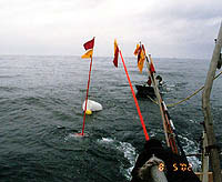 |
| Drogue deployment in Santa Monica Bay. Click to enlarge. |
May 2002 Analysis
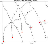 |
| Figure 3-1. Drogue tracking - courtesy of John Oram. Click to enlarge. |
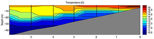 |
| Figure 3-2. Interpolated vertical temperature profiles. Inshore, temperatures are warmer with less stratification, while offshore, temperatures are lower with a greater degree of stratification. |
All plankton samples collected from the onshore-offshore transect were processed as above, and these data have been entered in tabular form in a spreadsheet where species abundances (identified to the lowest reasonable taxonomic level) were scored across stations. Early analysis indicates a strong association between water type and species assemblage.
July 2003 Cruise
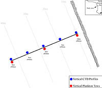 |
| Figure 3-3. Station Locations |
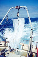 |
| Paired plankton nets. CTD (not clearly visible) is mounted between the mouth of the nets. Click to enlarge. |
Each day consisted of the following logistical approach. By 0800 we reoccupied the inner-most station and begin our transect heading out toward the outer-most station, while dropping our drogues in the water on the blue stations until they were all lined up on the transect (Figure 3-3). Once all the drogues were deployed, we would reverse course and perform CTD casts at the blue stations on the same original transect from the deepest to the shallowest station. Once inshore, we would then drive to each of the drogues and mark the time and their current position. After marking the drogues, we would then proceed to the original outer-most station (where the outer-most drogue was first dropped in the morning) and perform a CTD run back into shore. This process was repeated approximately every hour for 7 hours, giving me seven drogue readings and four to seven CTD runs along the transect. In addition to this, I collected vertical plankton tows at the red stations once during flood, once during slack, and once during ebb tide (a total of three sets of samples per day). As before, I used the paired plankton net equipped with General Oceanics flow meters. All samples were fixed in 4-5% formalin.
July 2003 Analysis
Data analysis for this chapter has just begun. A slick was observed throughout the day along the 10 m isobath, approximately 700 m outside the largest breakers. It persisted for most of the day, though the afternoon onshore winds (in excess of 10 kn) made it difficult to visualize. Preliminary profiles of CTD information for each transect are presented in Figure 3-4 for one of the three sampling days. Comparing these images over time has allowed me to detect changes in thermocline depth and possibly internal waves associated with the changing tide. Preliminary results of the drogue data indicate that the paths traveled by the drogues agree exactly with the information generated by the ADCP, and somewhat with the results of the May 2002 field effort. The inner-most drogue appeared to have moved almost entirely by tidal motion (Figure 3-5). However, the offshore drogues appear to also have been driven mostly by tides. This may be explained by the fact that all drogues were only submerged to a depth of 5 m, and the ADCP results (Figure 3-6) demonstrate the strongest water velocities were within the top 10 m of the water column. During flood tide, the surface water traveled in a northward direction (depicted in red), and then switched to a southward direction (depicted in blue) after the tide change. Velocities experienced in the vertical direction were negligible, with the highest values being much smaller than horizontal speeds by more than an order of magnitude.
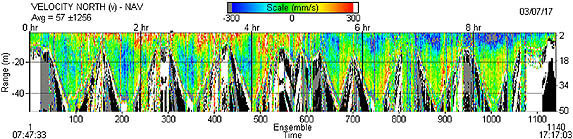 |
| Figure 3-6. Continuous vertical profile track of water velocity in the north direction from acoustic Doppler current profiler (ADCP) aboard the RV Seaworld UCLA from 07:47 to 17:17. Red color indicates water traveling to the north while blue color indicates water flowing to the south. White, black and gray color indicates the ocean bottom. Driving the boat repeatedly offshore and onshore gives the multi-humped shape to the graph. |
The ADCP clearly indicated that tides affected both the nearshore and offshore zones. However averaging the velocities in the nearshore zone (which was no more than 10m deep) and comparing them to averages of the upper 10 m of the offshore zone supports the drogue data in revealing that tides affect surface waters (in the upper 10 m) in a similar way regardless of distance from shore. However, since I did not submerge drogues in deeper water offshore, I cannot make a Eulerian comparison to the ADCP results.
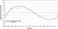 |
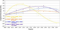
| Figure 3-7. Scatterplot and trend line of average longshore water velocity in the nearshore zone (averaged over entire depth - maximum depth = 10m). Positive values indicate longshore movement to the north. |
|
|
 |
| Figure 3-8. Scatterplot and trend line of average longshore water velocity in the offshore zone in four depth bins (yellow = 1-10m, orange = 11-20m, blue = 21-30m, and purple = 31-40m). Positive values indicate longshore movement to the north. |
Processing of plankton samples has commenced, and volumetric measurements have been recorded for all samples. Identification and enumeration of zooplankton will begin by mid-October, and data will be scored with multivariate statistics being utilized to establish any correlations between physical parameters and plankton abundance and diversity.
Non-parametric statistics will also be utilized to examine trends not addressable by multivariate statistics. For example, dissimilarity dendrograms generated for each day will illustrate degrees of dissimilarity between stations with respect to water type and species assemblage. The data will also be arranged in a grid for temporal analysis of changes in abundance and assemblage throughout a daytime tidal cycle.
Literature Cited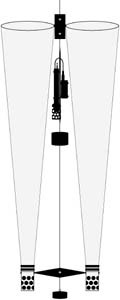
- Beer, T., 1983, Environmental Oceanography, An Introduction to the Behavior of Coastal Waters, Pergamon Press, NY.
- Brubaker, J., and R. Hooff, 2000, Limnol. Oceanogr. 45: 230-236.
- Carleton, J. H., R. Brinkman, and P.J. Doherty, 2001, Mar. Bio. 139: 705-717.
- Cowen, R. K., 2002, In: Coral Reef Fishes, Sale (ed.), Academic Press, San Diego, 149-170.
- Govoni, J. J., 1993, Bull. Mar. Sci. 53(2): 538-566.
- Jones, B. H., L. Washburn, Y. Wu, 1991, In: Coastal Zone 91: Proc. Seventh Sym. Coast. Ocean Manag., Amer. Soc. Civ. Engin., NY, 74-85.
- Jones, B. H., L. Washburn, S. Bay, K. Schiff, 1997, Proc. Cal. World Oceans Conf. 97., Amer. Soc. Civ. Engin., Reston, 24-27.
- Nakata, H., 1989, Rapp. pro.-ver. réun. 191: 153-159.
- Narcross, B. L., and R.F. Shaw, 1984, Trans. Amer. Fish. Soc. 113: 153-165.
- New, A. L., and R. D. Pingree, 1990, Deep-Sea Res. A – Oceanogr. Res. Pap. 37(12): 1783-1803.
- Oliver, J. K., B. L. Willis, 1987, Mar. Bio. 94: 521–529.
- Pingree, R. D., P. R. Pugh, P. M. Holligan, and G. R. Forster, 1975, Nature 258 (5537): 672-677.
- Sabatés, A., and M. Mas, 1990, Deep-Sea Res. 37: 1085-1098.
- Sakamoto, W., and Y. Tanaka, 1986, Bull. Japan. Soc. Sci. Fish. 52: 767-776.
- Shanks, A. L., 1983, Mar. Ecol. Prog. Ser. 13: 311-315.
- Shanks, A. L., 1985, Mar. Ecol. Prog. Ser. 24: 289-295.
- Shanks, A. L., 1986, Mar. Bio. 92: 189-199.
- Shanks, A. L., J. Largier, L. Brink, J. Brubaker, and R. Hooff, 2000, Limnol. Oceanogr. 45(1): 230-236.
- Wing, S.R., J.L. Largier, L.W. Botsford, J.F. Quinn, 1995, Limnol. Oceanogr. 40(2): 316-329.
- Wing, S. R., L. W. Botsford, J. L. Largier, L. E. Morgan, 1995, Mar. Ecol. Prog. Ser. 128: 199-211.
- Wolanski, E., 1994, Physical Oceanographic Processes of the Great Barrier Reef, CRC Press, Boca Raton, FL.
- Wolanski, E., and S. Sagnol, 2000, Estuar. Coast. Shelf Sci. 50: 27-32.
- Zeidberg, L. D., and W. M. Hamner, 2002, Mar. Bio. 141 (1): 111-122.
E-Mail - Kimo
Other Links
| Academic History | Diving History |
| Kimo's Home Page |
Copyright © 1996-2007, 2008 [A. Kimo Morris]. All rights reserved
Revised: January 7, 2006