Graduate work of A. Kimo Morris

The information below, is a follow-up study to an earlier field effort. For a brief introduction, please see the Initial Monterey study.

Sampling

On 22-24 August 2000, I revisited the Monterey upwelling front to perform a more detailed sampling effort aboard the Moss Landing vessel RV Ed Ricketts. With a better familiarity with the dynamics of the front, and a better understanding of how certain zooplankton assemblages might respond to the flow field, I was able to design a more extensive sampling array, with the addition of three more transects, and twenty one total samples. However the first three samples collected on 22 August were used only to identify the location of the front, and since the samples collected on the next two days overlapped these almost exactly, I did not used them in the analysis. Time, latitude, longitude, and depth were recorded at each station. 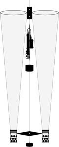Physical data were collected with a Seabird Electronics conductivity-temperature-depth (CTD) probe and also an Applied Microsystems Minibat towfish CTD fitted with a fluorometer. A paired plankton net, identical to that used in the April samples, was towed vertically at all stations. The Seabird CTD was mounted on the down cable below the mouth of the net openings, thus providing a vertical profile of depth, water temperature, salinity, and density. The Minibat was towed at the surface between stations to provide real-time data logging of chlorophyll a concentration and temperature.

AVHRR satellite images of sea surface temperature, downloaded from the Internet, were only available 12 hours after sampling. Therefore, I did not know the exact shape of the front at the precise sampling time. Thus, the physical properties of the water at any given station was not known to me in advance, although weekly averages leading up to the sampling days gave me a rough idea of the location of the front. SeaWiFS satellite images of chlorophyll concentration were available 14 days after sampling and were used as additional information of chlorophyll concentration.

Concurrent to the sampling on the RV Ed Ricketts, a remotely operated vehicle (ROV) deployed from the RV Pt. Lobos performed transects at night across the front. High-definition digital video transects recorded from the ROV Ventana were taken parallel and perpendicular to the front. This provided spatial information in situ on large macrozooplankton that are otherwise not adequately sampled with nets (Hamner et al., 1975). An onboard CTD provided physical information, and a global positioning system (GPS) and compass gave the location and orientation of the vehicle. All data were recorded to the video archive.

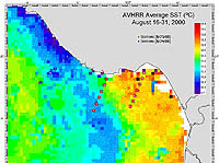Figure 2-3. AVHRR satellite image of sea surface temperature (click to enlarge)

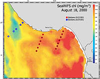Figure 2-4. SeaWiFS satellite image of chlorophyll-a concentration (click to enlarge)

As with the April cruise, samples were transferred into 0.1% formalin-seawater mixture in the lab. Sample volumes were measured (Kramer et al., 1972) and were split with a Folsam plankton splitter to a manageably sized aliquot (<3000 organisms per aliquot), and all animals were identified to the lowest reasonable taxonomic level. After identification and enumeration, non-gelatinous organisms were transferred to 70% ethanol, while gelatinous animals were preserved in 1% formalin-seawater, and voucher specimens were archived.

CTD data were downloaded and processed using Seasoft software and reduced using Microsoft Excel. Fluorometer data were downloaded with Applied Microsystems Smarttalk Software and reduced using Microsoft Excel. Both CTD and fluorometer data were then entered into Techplot software for graphing.

Station locations were plotted on a map, and SST (from AVHRR) and chlorophyll a concentration (SeaWiFS) satellite images were superimposed over the station map (Figure 2-3 and Figure 2-4, respectively). Again, this served to (a) verify that sampling indeed took place across the front, and (b) provide a comparison of in situ samples of sea surface temperature and surface chlorophyll a concentration.

Data were collected in a spatial array of known distances from each other, and physical information was gathered simultaneously to plankton tows. Therefore, a statistical correlative approach is an appropriate method to analyze these data. All data were entered into a matrix with enumerated species, biomass, all physical parameters and distance across stations. Since parametric statistics are generally more powerful than non-parametrics, I first separated my data into two groups – the first consisting of all normally distributed species for which I could perform parametric correlation statistic, and the second consisting of non-normally distributed species for which an appropriate non-parametric correlative approach could be utilized (Zar, 1984). A Kolmogrov-Smirnov test allowed me to separate my data into the two groups. For those species that were normally distributed, a Pearson correlation test was used to identify correlations between temperature and abundance. This initial exploratory approach revealed that certain species distributions are strongly correlated with water temperature, including ontogenic stages that don’t swim (e.g. euphausiids eggs), poor swimmers (e.g. the appendicularian Oikopleura spp.), as well as some species that are competent swimmers (e.g. the polychaete Magelona spp. and all ostracods). For those species distributed in a non-normal fashion, a Spearman rank order correlation was employed. As with the results of the Pearson correlation test, the Spearman rank order test showed significant correlations between water temperature and the distribution of certain species such as gastropod veligers and nemertine pilidium larvae, both considered relatively weak swimmers (Mileikovsky, 1973), and the proficient swimming ctenophore Pleurobrachia bachei. These preliminary data demonstrated that correlations do exist, and they also allowed me to exclude species from future analyses that have shown no relationship with temperature. The next step will be to take a more rigorous approach to the data. As my data are distributed spatially in a matrix of gradations, I have no real factor or treatment, and I therefore cannot perform typical traditional statistics (e.g. multivariate statistics). However, two approaches that are gaining in popularity in ecology and marine sciences in the past two decades that may prove useful include canonical correlation analysis (Coyle, 2000) and certain spatial autocorrelation techniques (Mackas, 1984; Kern and Coyle, 2000).

Data analysis for the gelatinous macrozooplankton transects is complete and shows a striking aggregation of the west coast sea nettle (Chrysaora fuscescens) along the front. From nine transects, we were able to draw strong correlations between jellyfish abundance and water mass type. Jellyfish were far more strongly associated with the nearshore warm water mass than with the colder offshore upwelled water. In addition, no matter where jellyfish were located in the vicinity of the front, virtually all exhibited a swimming behavior that oriented them towards the front. Thus, these neurologically simple animals are apparently able to respond to their environment in a way that optimizes feeding, since the zooplankton they eat are also highly aggregated along the front.

Data Interpretation

Throughout the cruise, wind speeds varied with location. Winds tended to be less than 12 kn southward in the vicinity of the two east-most transects, while wind speeds often exceeded 15kn in waters near the west-most transect. A front was seen perpendicular to the west-most transect, though it was not as sharp a barrier as was seen in the previous survey. No fronts were visualized near the two east-most transects, though CTD and satellite data indicate that they were run through horizontal gradients in temperature and chlorophyll a concentration (Figure 2-8, results only for the middle transect B off Santa Cruz, see Figure 2-3 for transect location).

Preliminary data analysis looks promising with strong correlations noted between certain species and temperature. What is most compelling is that the association is not exclusive to passively transported zooplankton, such as fish eggs or euphausiids eggs. Rather, many organisms with differing degrees of swimming competence are found strongly associated with certain water types. While clearly more rigorous testing is necessary to draw stronger conclusions, the preliminary results suggest that stronger swimming zooplankton may be aggregating in the richer feed zones associated with the cooler nutrient-rich upwelled water. However, a robust analysis using a canonical correlation or spatial autocorrelation technique will be necessary to test such a hypothesis. Larval crustaceans do not show strong correlations with the physical data, however crab larvae (presumably also larval shrimp) are located at different depths within the water column at various times throughout a 24-hour period of time (e.g. Shanks, 1986). It is possible that since my data were collected only during an 8-hour period of time during the day, and since my vertical tows may have under-sampled particular depth bins, I may not have enough information to address larval crustacean distributions. Therefore, the apparent lack of association between larval crustacean distributions and physical water properties may more likely be due to inadequate sampling methodology of larval crustaceans.

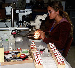UCLA undergraduate Anne Elise Nieblas assumes the position at the scope! I owe a debt of gratitude to all the assistants for their hard work and dedication to this project.

• Coyle, K.O., 2000, Can. J. Fish. Aqu. Sci. 57(11): 2306-2318.
• Hamner, W.M., L.P. Madin, A.L. Alldredge, R.W. Gilmer, and P.P. Hamner, 1975, Limnol. Ocean. 20(6): 907-917.
• Kern, J.W., and K.O. Coyle, 2000, Can. J. Fish. Aqu. Sci. 57(10): 2112-2121.
• Kramer, D., M.J. Kalin, E.G. Stevens, J.R. Thrailkill, J.R. Zweifel, 1972, NOAA Tech. Report NMFS CIRC-370, Seattle WA.
• Mackas, D.L., 1984, Limnol. Ocean. 29(3): 451-471.
• Mileikovsky, S.A., 1973, Mar. Bio. 23: 11-17.
• Shanks, A.L., 1986, Mar. Bio. 92: 189-199.
• Zar, J.H. 1984. Biostatistical Analysis. Prentice-Hall. Englewood Cliffs, NJ.